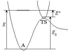
Fig. 4.1

- Microcanonical form of the Transition State Theory
Fig. 4.1
[ ]
]
 (4.1.1)
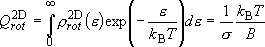
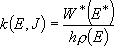
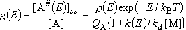
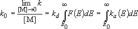
Microcanonical equilibrium :
( :
1-D translational energy of TS)
:
1-D translational energy of TS)
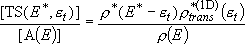 (4.1.2)
Half of  passes region
with length
passes region
with length  toward products
with velocity
toward products
with velocity  .
.
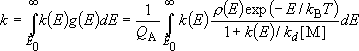
 rate of reaction :
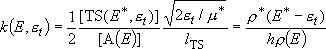
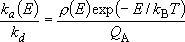
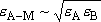
Rate coefficients for A( ) :
) :
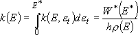 (4.1.3)
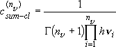
 [sum of states] (4.1.4)
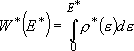
by taking adiabatic rotation into account;
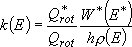 (4.1.5)
or 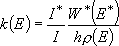 (4.1.5')
 (4.1.6)
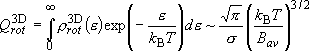 (4.1.7)
note:
Exactly speaking, eq. (4.1.5) is not a correct form of the
microscopic rate coefficient. see
appendix for detail.
|
Problem-4.1 [OPTION] Derive eqs. (4.1.6) and (4.1.7) from eqs. (2.2.7) and (2.2.10). |
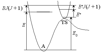
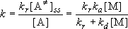
Fig. 4.2 
[ ]
]
- Conservation of angular momentum
 (4.1.8)
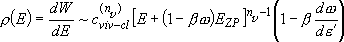
Microscopic rate coefficients:
 (4.1.9)
note:
For the case of similar structures of A and TS (i.e.,


 )
)
 -conservation may be
ignored.
-conservation may be
ignored.
[Sum of states]
summationintegration (2.3.5)
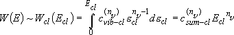 (4.1.10)
 ,
,
note:
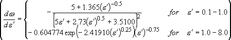
Classical approximation [(2.3.5) , (4.1.10)] :
Not good at low energy (fig. 2)
Whitten-Rabinovitch Approximation or
Direct Count
[Whitten-Rabinovich Approximation]
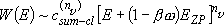 (4.1.11)
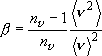 ,
,
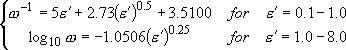 ,
,

 (4.1.12)
[Direct Count (Beyer-Swinehart algorithm)]
Count states in energy grains (source list 1)
Stein & Rabinovitch, J. Chem. Phys.
58, 2438 (1973).
|
Problem-4.2
1) Evaluate
2) [OPTION] Evaluate the density/sum of states by direct count, and compare with above results. | |||||||||||||
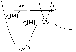
Fig. 4.3 Lindemann-Mechanism
[Lindemann Mechanism] (review)
Steady-state assumption for [ ]
]
 (4.2.1)
High-pressure limit :
 (4.2.2)
Low-pressure limit :
 (4.2.3)
 (4.2.4)
Fall-off pressure (density) :
 (4.2.5)
note:
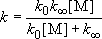
- Eq. (4.2.4) cannot reproduce the measurements (fig. 4.4)
since is not a single state.
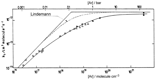
Fig. 4.4 Rate constant for CH3 + O2
recombination reaction
[Troe's formula]
- semi-empirical / reproduces measurements
[a] J. Troe, J. Phys. Chem. 83, 114
(1979).
[b] R. G. Gilbert, K. Luther, and J. Troe, Ber.
Bunsenges. Phys. Chem. 87, 169 (1983).
 (4.2.6)
 ,
,
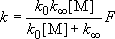
 [a] (4.2.7)
 ,
,
 ,
,
 ,
,
 [a] (4.2.8)
(4.1.5), (4.1.9) Microcanonical form
of RRKM theory
['Lindemann' to RRKM]
 ,
,
 ,
,
 ,
[
,
[ :
a constant independent of ]
:
a constant independent of ]
Detailed balancing :
 (4.3.1)
steady-state assumption to 
distribution function :
 (4.3.2)
 (4.3.3)
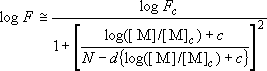
[High-pressure limit] = canonical average = TST (transition-state theory)
Canonical (Boltzmann) distribution of
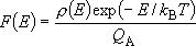 (4.3.4)
(4.3.2)  ...
...

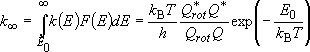 = TST
(4.3.5)
= TST
(4.3.5)
|
Problem-4.3 Derive the eq. (4.3.5) by using
in eq. (4.1.5).
|
[Low-pressure limit] = excitation is rate-determining
(4.3.3)  :
:
 (4.3.6)
note :
- Fall-off region low-pressure limit
: Vibrational distribution is non-Boltzmann
[Strong-collision RRKM theory]
assumption : of
 deactivates to
 by a single collision with M.
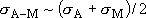
Lennard-Jones collision frequency :
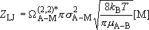 (4.3.7)
Strong-collision deactivation rate coefficient :
 (4.3.8)
or 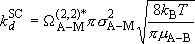
 ,
,
 ,
,
 :
:
(4.3.3)
 ,
(4.3.6)
,
(4.3.6)
 ,
(4.3.2)
,
(4.3.2)

[Weak-collision correction]
- Strong collision RRKM > measurements @ fall-off
low-pressure limit
 (4.3.9)
 :
weak collision parameter 0.1 1
(depending on temperature, molecule, M)
:
weak collision parameter 0.1 1
(depending on temperature, molecule, M)
 :
:
(4.3.3)
 ,
(4.3.6)
,
(4.3.6)
 ,
(4.3.2)
,
(4.3.2)

|
Problem-4.4 [OPTION] 1) By using the weak collision corrected RRKM theory, calculate  , ,
 ,
and ,
and  at at  at 800 K for
the reaction in the problem-4.2. Calculate at 800 K for
the reaction in the problem-4.2. Calculate  and
and  by the Whitten-Rabinovich approximation or
by the direct count. Assume
= 0.2 and M = Ar, and use by the Whitten-Rabinovich approximation or
by the direct count. Assume
= 0.2 and M = Ar, and use
 (CH3CH2I) = 5.3 (CH3CH2I) = 5.3
 , (Ar) = 3.5
, , (Ar) = 3.5
,
 (CH3CH2I) /
B = 320 K, and
(Ar) / B
= 93 K. (CH3CH2I) /
B = 320 K, and
(Ar) / B
= 93 K.2) Plot the weak collision vibrational energy distribution, , at against
, and compare it with the Boltzmann
distribution,  . .
|
[Master Equation-RRKM]
WC-RRKM :
- Satisfactory in many cases, but
has little physical
meaning.
- Cannot describe multi-channel / multi-well problems.
Master equation system describing the problem :
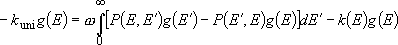 (4.3.10)
 :
(steady-state) unimolecular reaction rate coefficients,
:
(steady-state) unimolecular reaction rate coefficients,
 : collision frequency;
[=
: collision frequency;
[=  (4.3.7)],
 or
or
 : probability of energy
transfer (from
: probability of energy
transfer (from  to ,
or to )
to ,
or to )
By using energy grain matrix form :
 (4.3.11)
... eigenvalue problem of matrix
 .
Compare the results of classical approximation [(2.3.5), (4.1.10)] and
Whitten-Rabinovitch approximation [(4.1.11), (4.1.12)].
.
Compare the results of classical approximation [(2.3.5), (4.1.10)] and
Whitten-Rabinovitch approximation [(4.1.11), (4.1.12)]. = 17800