Using Octave - Introduction to Octave
A. Miyoshi
A. Miyoshi
GNU Octave is a high-level programming language (freeware) for scientific computation developed by John W. Eaton and others. This instruction is based on the Octave 4.2.2 as of March 2018. Please understand that some information may not be up-to-date due to the improvement and/or update.
 Official site instructs downloading and installing Octave
for various operating systems (GNU/Linux. macOS, BSD, and Windows).
 Official Manual The number of users has been
increased in the last decade, and the search on the web has become useful
to find some answers.
octave↵ in the command line.
GNU Octave, version 4.2.2
Copyright (C) 2018 John W. Eaton and others.
 :
>>
exit↵
or quit↵ on the prompt of
Octave. ( >> ). Underline denotes the key-in part, and
"↵" denotes [Enter] key.
>> exit↵
>> 2.3 * exp(-0.23 * 2)↵
ans =  1.4520
format long↵
to increase the significant
digits for output. It also can be specified by the
number of significant digits with
output_precision(12)↵ .
>> 5 * ans↵
ans =  7.2598
>> format long↵
>> ans↵
ans = 7.25976192332965
>> output_precision(12)↵
>> ans↵
ans =  7.25976192333
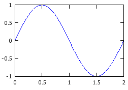
>> x = 0:0.01:2;↵
>> plot (x, sin(pi*x));↵

mysource.m, with the following contents in the current directory
of the running Octave.
x = 1:10
sum(x)
>> mysource↵
x =
    1    2    3    4    5    6    7    8    9   10
ans =  55
source
function. The only one difference from above is that the
extension of the file name should not be ".m".
>> source mysource.m↵
edit function.
>> edit mysource.m↵
~/.octave_hist (UNIX including WSL) or
C:\Users\user_name\.octave_hist (Windows).
[ ] in which semicolon
";" is used as a line delimiter and a white space
" " or a comma ","
is used as a column delimiter. In the following example,
a linear equation system, Ax = b, is solved.
>> A = [2, 1; 1, 3]↵
A =
   2   1
   1   3
>> b = [3; 4]↵
b =
   3
   4
>> x = A \ b↵
x =
   1.00000
   1.00000
inv() function to calculate inverse
matrix, or by using the postfix operator '
to denote transposition.
>> inv(A)↵
ans =
   0.60000  -0.20000
  -0.20000   0.40000
>> b'↵
ans =
   3   4
>> b' * b↵
ans =  25
>> det(A)↵
ans =  5.0000
lambda as diagonal elements in the descending
order, and eigenvectors are stored in a matrix vec
as vertical vectors in the same order as eigenvalues.
>> A = [-1, 1; 1, -1]↵
A =
  -1   1
   1  -1
>> [vec, lambda] = eig(A)↵
vec =
   0.70711   0.70711
  -0.70711   0.70711
lambda =
Diagonal Matrix
  -2   0
   0   0
f.
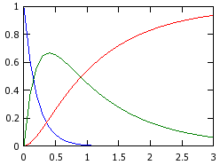
>> function xdot = f(x, t)↵
  xdot(1) = -5 * x(1);↵
  xdot(2) =  5 * x(1) - 1 * x(2);↵
  xdot(3) =             1 * x(2);↵
endfunction↵
x0, and the output times,
t.
linspace is a function which generates a sequence of numbers with a
constant interval as a row vector.
>> x0 = [1; 0; 0];↵
>> t = linspace(0, 3, 31)';↵
lsode.
>> xout = lsode("f", x0, t);↵
t, appended as the
first column.
format is a function to define output format.
[t, xout] is a combined matrix of column vector t and
the matrix, xout, with the same number of rows.
>> format short;↵
>> [t, xout]↵
ans =
   0.00000   1.00000   0.00000   0.00000
   0.10000   0.60653   0.37288   0.02059
     :         :         :         :
   3.00000   0.00000   0.06223   0.93777
>> plot(t, xout)↵

fsolve function is a solver for nonlinear
equations in Octave. The example below solves the following
nonlinear equation.
f
so that the nonlinear equation to be solved is f(x) = 0.
>> function y = f(x)↵
>   y = 1e13 * x^(-1.39) * exp(-17921/x) - 1;↵
> endfunction↵
fsolve with
the initial guess of the solution.
>> [x, fval, info] = fsolve("f", 800)↵
x =  873.34
fval = 9.4820e-007
info =  1
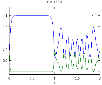
>> gray_scott↵If you do not know where is the current directory, try typing
pwd↵.
>> pwd↵
ans = C:\Users\myaccount
