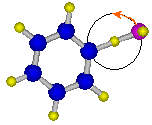
Fig. QS2-1. "Wagging" vibraion of H-abstraction TS of OH + benzene.
Having succeeded to run BEx1D tools, let us investigate the sample input and ouput files in detail in the next three steps.
Sample problem 1: wagOHbenTSabs

bx1fitPlls input: wagOHbenTSabs.fit
'#' is a title line:# CH-OH wag of OH + benzene H abstraction TS (mass weighted coordinate)
outputOption powerSerieswhich tells bx1fitPlls to generate input file for bx1VIBsol named
'wagOHbenTSabs.inp'. Note that bx1VIBsol only
accept power series potential and the regression function defined
in the following block must be a power series.
optFuncs{
  const
  pow   2
  pow   4
  pow   6
  pow   8
  pow  10
  pow  12
}
defines the regression function. The key 'const'
stands for a constant term, and 'pow n' means
xn. Thus, this example is a
polynomial;
y = a0
+ a1x2
+ a2x4
+ a3x6
+ a4x8
+ a5x10.
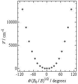
xyTable{
  0.           0.
  0.175395353  40.11886525
  0.354069718  189.0859545
  0.538962708  521.7658202
  0.73251983   1134.26377
  0.936579205  2136.432343
  1.152654481  3654.297605
  1.382347157  5833.785823
  1.627451293  8827.658145
  1.889951279  12732.18273
}
where each line in the block beginning with 'xyTable{' terminating
by '}' contains one datum point, in the order of x (coordinate)
and y (potential energy). As shown in Fig. QS2-2, the
potential energy curve is anharmonic.
continue{
 numBasis  501     ! number of basis functions
 rotConst  1.89349 ! rotational constant [cm-1]
 hoFreq    73.3072 ! harmonic oscillator frequency [cm-1]
 !
 ! output vector   ! (and/or function)
 !
  tempRange 300 570 30
  tempRange 600 950 50
  tempRange 1000 2000 100
}
Any line in this block is merely copied to the bx1VIBsol input,
'wagOHbenTSabs.inp'. Although bx1fitPlls neither
reads nor checks the contents of this block, they must be proper
input for bx1VIBsol.bx1fitPlls console output
'wagOHbenTSabs.inp'. Other
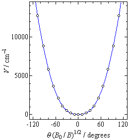
diagnostic messages and related statistics are printed to the console.===== results of linear least squares regression ===== Function: y = a0 + a1 * x^2 + a2 * x^4 + a3 * x^6 + a4 * x^8 + a5 * x^10 + a6 * x^12The parameters to be optimized are numbered consecutively,
a0, a1, a2, ..., as they
appear in the optFuncs block.Optimum parameters (+-) standard deviations (relative) a0 = -1.0306367e+000 (+-) 1.3167189e+000 ( 127.76 %) a1 = 1.2877844e+003 (+-) 2.0212666e+001 ( 1.57 %) a2 = 2.0746208e+003 (+-) 7.4216348e+001 ( 3.58 %) a3 = -1.2492067e+003 (+-) 1.0363676e+002 ( 8.30 %) a4 = 5.3098393e+002 (+-) 6.5249151e+001 ( 12.29 %) a5 = -1.2179626e+002 (+-) 1.8647156e+001 ( 15.31 %) a6 = 1.1063236e+001 (+-) 1.9588634e+000 ( 17.71 %)show the optimum parameters and their estimated errors.
 Parameter correlation coefficients
            a0       a1       a2       a3       a4       a5
  a1  -0.68038
  a2   0.53582 -0.95926
  a3  -0.46231  0.90454 -0.98652
  a4   0.41867 -0.85999  0.96386 -0.99420
  a5  -0.39058  0.82631 -0.94249  0.98355 -0.99721
  a6   0.37162 -0.80129  0.92476 -0.97281  0.99186 -0.99858
wagOHbenTSabs.inpwagOHbenTSabs.fit:# CH-OH wag of OH + benzene H abstraction TS (mass weighted coordinate)
continue
block contents:numBasis 501 ! number of basis functions rotConst 1.89349 ! rotational constant [cm-1] hoFreq 73.3072 ! harmonic oscillator frequency [cm-1] ! ! output vector ! (and/or function) ! tempRange 300 570 30 tempRange 600 950 50 tempRange 1000 2000 100In this example, number of basis functions (
numBasis)
is 501, meaning that the harmonic oscillator basis functions (so-called
Hermite-Gaussian functions) for quantum number 0 to 500 are used as
the expansion basis. The next key, rotConst (or
equivalently, hbar2/2m), sets the rotational constant
( = hoFreq, the harmonic
oscillator frequency, input.output key input. This key controls
the output of bex1VIBsol.
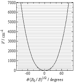
potPars{           ! potential parameters
  0   -1.0306367
  2   1287.7844
  4   2074.6208
  6   -1249.2067
  8   530.98393
  10   -121.79626
  12   11.063236
}
Each line in the block specifies the order ni and
coefficient ai for the power series term,
aixni. 'wagOHbenTSabs_eigen_values.csv' (eigen values) and
'wagOHbenTSabs_part_funcs.csv' (partition functions).
Optionally, by setting the output key in the input,
'wagOHbenTSabs_eigen_vectors00.csv' (eigen vectors)
and 'wagOHbenTSabs_eigen_funcs00.csv' (eigen functions)
will be also created.
| number | eigenValue | w |
| 0 | 50.340893 | (1/1) |
| 1 | 156.5024 | (1/1) |
| 2 | 268.75298 | (1/1) |
| 3 | 385.86919 | (1/1) |
| 4 | 507.03996 | (1/1) |
| 5 | 631.67864 | (1/1) |
| 6 | 759.33796 | (1/1) |
| 7 | 889.66457 | (1/1) |
| 8 | 1022.3721 | (1/1) |
| ... | ... | ... |
| 10000/T | T | Q |
| 33.333333 | 300 | 1.882205 |
| 30.30303 | 330 | 2.0603718 |
| 27.777778 | 360 | 2.2366488 |
| 25.641026 | 390 | 2.4112197 |
| 23.809524 | 420 | 2.5842349 |
| ... | ... | ... |